One crucial boundary condition for such models is the time-varying tendencies of heat and moisture from horizontal and vertical advection. Due to the difficulty of directly obtaining these tendencies, we instead provide hourly tendencies from short-range (12-35 hour) forecasts at the moving SHEBA column position provided by ECMWF. These forecasts assimilated SHEBA rawinsonde soundings and surface observations , and are generally in good agreement with the observed soundings. You may also link to a larger netcdf file containing a complete suite of hourly output from the ECMWF model.

Other datasets include all rawinsonde soundings , and hourly-averaged data from lidar, radar , meteorological surface observations and a microwave radiometer. An overall discussion of many of these measurements and how they compare with the ECMWF predictions can be found in:

Bretherton, C. S., S. R. de Roode, C. Jakob, E. A. Andreas, J. Intrieri, R. E. Moritz, and P. O. G. Persson, 2000: A comparison of the ECMWF forecast model with observations over the annual cycle at SHEBA. Revised version submitted to the special FIREIII issue of the Journal of Geophysical Research, May 2000. (Postscript version)

Below, we summarize the different variables we have compiled. We include two tables: first those relevant to model initialization and boundary conditions, and second the available variables for model verification. Turbulence and tower observations made during May 1998 by the group of Peter Duynkerke (2000) have been archived too, as this period is of special interest as a SHEBA/FIRE.ACE intensive observing period.

A single-column model can be initialized using the rawinsonde observations, whereas boundary conditions such as horizontal and vertical advection can be taken from the ECMWF model predictions. Moreover, continuous surface observations provide information such as surface albedo, surface pressure and/or turbulent surface fluxes. The following table summarizes the major variables that are needed for model initialization and horizontal and surface boundary conditions, and the names of the files in which they are stored.

(*1) The downward-pointing pyranometer at the flux tower measured upwelling shortwave radiation from a small area that mainly consisted of bare ice during the summer melt season. The surface albedo calculated from this measurement ('tower_albedo') was similar to other SHEBA estimates (line-averaged or aerial estimates that averaged across a variety of surface types) in the winter, but up to 15% higher at times in the late summer.

Thus the effect of adiabatic compression/expansion is included in this term.

Vertical profiles of variables like temperature can also be taken from the ECMWF model predictions. However, care should be taken about the model-predicted atmospheric boundary layer structure. In particular during the Arctic winter season the ECMWF surface temperatures sometimes significantly differed from the tower observations. This can be attributed to the sea-ice model which treated sea-ice as an isothermal slab, which dramatically damped day-to-day surface air temperature fluctuations compared to the observations, creating 10-15 K errors in surface air temperature, particularly under clear calm conditions.

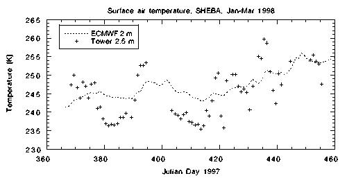Observed and ECMWF model-predicted near surface temperature, for January-March 1998 (Bretherton et al. 2000, Fig. 1a)

Moreover, sharp temperature inversions capping the boundary layer were frequently observed. Because of of its rather coarse resolution the ECMWF model tends to smear this profile out.

 

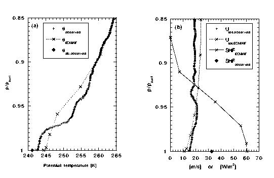Example of a rawinsonde sounding and ECMWF model results for 12 UTC 21 February 1998. (a) shows the model and observed potential temperature and (b) the model and observed winds and model downward turbulent heat fluxes. The diamond marks indicate the observed surface potential temperature (left panel) and observed downward sensible heat flux (right panel) (Bretherton et al. 2000, Fig. 6).

 

Observations of the surface turbulent heat fluxes and radiation can be used to verify the surface energy balance. Microwave radiometer retrievals provide the water vapor and liquid water paths, and lidar and radar data give information about cloud presence and cloud phase. The following table summarizes the major variables that are needed for model verification and the names of the files in which they are stored.

 

VARIABLE	netCDF VARIABLE NAME	FILE NAME
Temperature	nc{'temp'}	rawinsonde.nc
Relative humidity	nc{'rh'}	rawinsonde.nc
Wind velocity	nc{'wtot'}	rawinsonde.nc
Wind direction	nc{'wdir'}	rawinsonde.nc
Surface temperature	nc{'T_sfc'}	surf_obs.nc
Sensible heat flux	nc{'hs'}	surf_obs.nc
Latent heat flux	nc{'hlb_2_5'}	surf_obs.nc
ustar	nc{'ustar'}	surf_obs.nc
Upward longwave flux	nc{'LWu'}	surf_obs.nc
Downward longwave flux	nc{'LWd'}	surf_obs.nc
Upward shortwave flux	nc{'SWu'} / nc{'SWucor'}	surf_obs.nc
Downward shortwave flux	nc{'SWd'}	surf_obs.nc
Liquid water path	nc{'lwp'}	surf_obs.nc
Water vapor path	nc{'wvp'}	surf_obs.nc
Cloud reflectivity	nc{'dBZ'}	radarhh.nc
Cloud base height	nc{'altitude'}	lidardata.nc
depolarization (indication of cloud phase)	nc{'depol'}	lidardata.nc

 

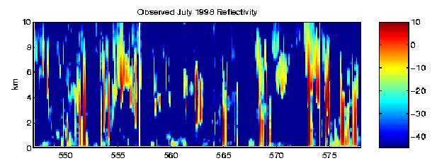Observed radar reflectivities for July 1998 (Bretherton et al. 2000, Fig. 9).